Prediction of the 10-year Cardiovascular Heart Disease
Using the Framingham Heart Study Data
Chapter 5. Model Evaluation
In the previous Chapter, we have checked the accuracy of four different models.
To recap, the accuracy LogisticRegression was highest (68.35%), followed by SVC (65.82), KNeighbors (56.12%),
and DecisionTree (54.01%). Accuracy is one of several measures to check the model's validity.
In this Chapter, we assess each model and select the best one for our prediction of 10-year CHD
using the Framingham Heart Study data.
1. Logistic Regression
Logistic regression, a fundamental concept in both machine learning and statistics, plays a pivotal
role in predicting binary outcomes. In the realm of machine learning, logistic regression is an
algorithmic technique that falls under supervised learning. It harnesses the power of mathematical
optimization to estimate the probability of an event occurring within a given set of independent
variables. By modeling this relationship using a logistic function, it effectively classifies
data points into distinct categories based on their features.
In traditional statistics, logistic regression serves as an inferential tool allowing researchers to
analyze relationships between predictor variables and categorical response variables. By employing
maximum likelihood estimation methods or alternative statistical techniques such as Wald tests or odds
ratios, statisticians can interpret coefficients to assess significance levels and make reliable
predictions regarding factors influencing an outcome variable's occurrence or absence.
While both disciplines utilize logistic regression for prediction purposes, they may differ in terms
of methodologies employed and degree of emphasis placed on interpretability versus predictive accuracy.
We are using the normalized data again. First import libraries
from sklearn.model_selection import cross_val_score
from sklearn.metrics import confusion_matrix
from sklearn.metrics import accuracy_score
from sklearn.metrics import f1_score
from sklearn.metrics import recall_score
from sklearn.metrics import precision_score
from sklearn.metrics import roc_curve
from sklearn.metrics import roc_auc_score
normalized_df_reg = LogisticRegression().fit(X_train, y_train)
normalized_df_reg_pred = normalized_df_reg.predict(X_test)
# check accuracy: Accuracy: Overall, how often is the classifier correct?
Accuracy = (True Pos + True Negative)/total
acc = accuracy_score(y_test, normalized_df_reg_pred)
print(f"The accuracy score for LogReg is: {round(acc,3)*100}%")
F-1 score:
The F-1 score is an essential metric in machine learning that provides a balanced measure of a model's accuracy. It can be interpreted as a weighted average of the precision and recall. It serves as a comprehensive evaluation criterion to assess the effectiveness of classification algorithms. The F-1 score achieves this by harmonizing precision, which represents the proportion of correctly identified positive instances out of all predicted positives, with recall, denoting the ratio of correctly classified positive instances out of all actual positives.
As such, it effectively captures how well a model can detect relevant data points while minimizing false positives or negatives. By striking a balance between these two vital aspects, the F-1 score allows for more informed decisions when comparing and selecting machine learning models across various domains and applications.
f1 = f1_score(y_test, normalized_df_reg_pred)
print(f"The f1 score for Logistic Regression is: {round(f1,3)*100}%")
Output:
The f1 score for Logistic Regression is: 67.0%
Precision score:
When it predicts yes, how often is it correct? Precision=True Positive/predicted yes
precision = precision_score(y_test, normalized_df_reg_pred)
print(f"The precision score for LogReg is: {round(precision,3)*100}%")
Output:
The precision score for Logistic Regression is: 65.0%
Recall score:
True Positive Rate(Sensitivity or Recall): When it’s actually yes, how often does it predict yes? True Positive Rate = True Positive/actual yes
recall = recall_score(y_test, normalized_df_reg_pred)
print(f"The recall score for LogReg is: {round(recall,3)*100}%")
Output:
The recall score for LogReg is: 69.1%
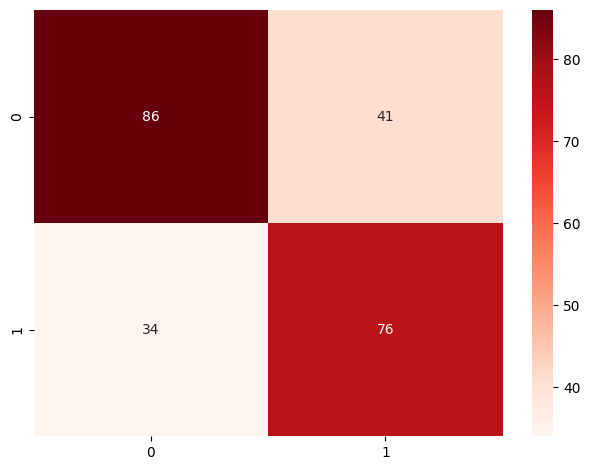
plotting confusion matrix Logistic Regression
cnf_matrix_log = confusion_matrix(y_test, normalized_df_reg_pred)
Confusion matrix graph
fig, ax = plt.subplots()
sns.heatmap(pd.DataFrame(cnf_matrix_log), annot=True,cmap="Reds" , fmt='g')
ax.xaxis.set_label_position("top")
plt.tight_layout()
plt.savefig('./static/image/confusion_logistic', bbox_inches='tight')
# plt.title('Confusion matrix Logistic Regression\n', y=1.1)
plt.show()
Figure 1. Confustion matrix

2. Support Vector Machine (SVM)
svm = SVC() #initialize model
svm.fit(X_train, y_train) #fit model
normalized_df_svm_pred = svm.predict(X_test)
Accuracy Score:
Accuracy: Overall, how often is the classifier correct? Accuracy = (True Pos + True Negative)/total
acc = accuracy_score(y_test, normalized_df_svm_pred)
print(f"The accuracy score for SVM is: {round(acc,3)*100}%")
Output:
The accuracy score for SVM is: 65.8%
# f1 score:
The F1 score can be interpreted as a weighted average of the precision and recall, where an F1 score reaches
its best value at 1 and worst score at 0.
f1 = f1_score(y_test, normalized_df_svm_pred)
  print(f"The f1 score for SVM is: {round(f1,3)*100}%")
Output:
The f1 score for SVM is: 63.7%
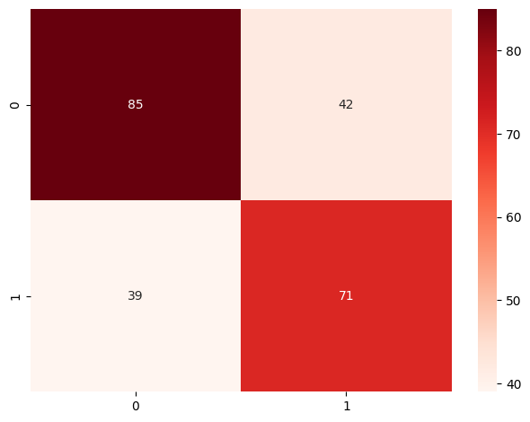
# plotting confusion matrix SVM
cnf_matrix_svm = confusion_matrix(y_test, normalized_df_svm_pred)
sns.heatmap(pd.DataFrame(cnf_matrix_svm), annot=True,cmap="Reds" , fmt='g')
ax.xaxis.set_label_position("top")
plt.tight_layout()
# plt.title('Confusion matrix SVM\n', y=1.1)
plt.show()
Figure 2. Confusion matrix - SVM

3. Decision Tree
# initialize model
dtc_up = DecisionTreeClassifier()
# fit model
dtc_up.fit(X_train, y_train)
normalized_df_dtc_pred = dtc_up.predict(X_test)
Accuracy
# Overall, how often is the classifier correct? Accuracy = (True Pos + True Negative)/total
acc = accuracy_score(y_test, normalized_df_dtc_pred)
print(f"The accuracy score for DTC is: {round(acc,3)*100}%")
Output:
The accuracy score for DTC is: 53.2%
f1 score
The F1 score can be interpreted as a weighted average of the precision and recall, where an F1 score
reaches its best value at 1 and worst score at 0.
f1 = f1_score(y_test, normalized_df_dtc_pred)
print(f"The f1 score for DTC is: {round(f1,3)*100}%")
Output:
The f1 score for DTC is: 48.8%
Precision score:
When it predicts yes, how often is it correct? Precision=True Positive/predicted yes
precision = precision_score(y_test, normalized_df_dtc_pred)
print(f"The precision score for DTC is: {round(precision, 3)*100}%")
Output:
The precision score for DTC is: 49.5%
recall score:
True Positive Rate(Sensitivity or Recall): When it’s actually yes, how often does it predict yes?
True Positive Rate = True Positive/actual yes
Output:
The recall score for DTC is: 48.20%
# plotting confusion matrix Decision Tree
cnf_matrix_dtc = confusion_matrix(y_test, normalized_df_dtc_pred)
sns.heatmap(pd.DataFrame(cnf_matrix_dtc), annot=True,cmap="Reds" , fmt='g')
ax.xaxis.set_label_position("top")
plt.tight_layout()
plt.show()
Figure 3. Confusion matrix Decision Tree

4. KNN Model
knn = KNeighborsClassifier(n_neighbors = 2) # initialize model
knn.fit(X_train, y_train) # fit model
normalized_df_knn_pred = knn.predict(X_test)
Accuracy:
Overall, how often is the classifier correct? Accuracy = (True Pos + True Negative)/total
acc = accuracy_score(y_test, normalized_df_knn_pred)
print(f"The accuracy score for KNN is: {round(acc, 3)*100}%")
Output:
The accuracy score for KNN is: 61.2%
f1 score:
The F1 score can be interpreted as a weighted average of the precision and recall,
where an F1 score reaches its best value at 1 and worst score at 0.
f1 = f1_score(y_test, normalized_df_knn_pred)
print(f"The f1 score for KNN is: {round(f1, 3) * 100}%")
Output:
The f1 score for KNN is: 46.5%
Precision score:
When it predicts yes, how often is it correct? Precision=True Positive/predicted yes
precision = precision_score(y_test, normalized_df_knn_pred)

print(f"The precision score for KNN is: {round(precision, 3)*100}%")
Output:
The precision score for KNN is: 64.5%
recall score:
True Positive Rate(Sensitivity or Recall): When it’s actually yes, how often does it predict yes?
True Positive Rate = True Positive/actual yes
recall = recall_score(y_test, normalized_df_knn_pred)

print(f"The recall score for KNN is: {round(recall, 3) * 100}%")
Output:
The recall score for KNN is: 36.4%
Result: The KNN model has the highest accuracy score.
# Check overfit of the KNN model
# accuracy test and train
acc_test = knn.score(X_test, y_test)
print("The accuracy score of the test data is: ", acc_test * 100,"%")
acc_train = knn.score(X_train, y_train)
print("The accuracy score of the training data is: ", round(acc_train * 100, 2),"%")
Output:
The accuracy score of the test data is: 61.2%
The accuracy score of the training data is: 79.1%
# The scores for test and training data for the KNN model are similar.
Therefore, we do not expect the model to overfit.
Perform cross validation
Cross Validation is used to assess the predictive performance of the models and to judge
how they perform outside the sample to a new data set.
cv_results = cross_val_score(knn, X, y, cv=5)
print ("Cross-validated scores:", cv_results)
print("The Accuracy of Model with Cross Validation is: {0:.2f}%".format(cv_results.mean() * 100))
Output:
Cross-validated scores: [0.62025316 0.56962025 0.5720339 0.61016949 0.61864407]
The Accuracy of Model with Cross Validation is: 59.81%
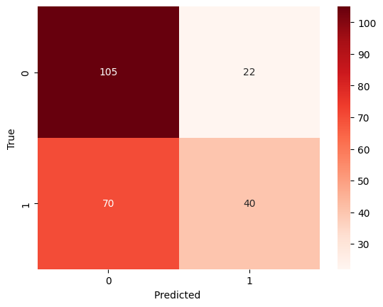
# plotting confusion matrix KNN
cnf_matrix_knn = confusion_matrix(y_test, normalized_df_knn_pred)
ax= plt.subplot()
sns.heatmap(pd.DataFrame(cnf_matrix_knn), annot=True,cmap="Reds" , fmt='g')
ax.set_xlabel('Predicted ');ax.set_ylabel('True')
plt.show()
Figure 5. Confusion matrix - KNN

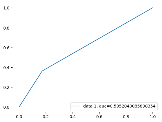
#AU ROC CURVE KNN
'''the AUC ROC Curve is a measure of performance based on plotting the true positive and false positive
rate and calculating the area under that curve.The closer the score to 1 the better the algorithm's
ability to distinguish between the two outcome classes.'''
fpr, tpr, _ = roc_curve(y_test, normalized_df_knn_pred)
auc = roc_auc_score(y_test, normalized_df_knn_pred)
plt.plot(fpr,tpr,label="data 1, auc="+str(auc))
plt.legend(loc=4)
plt.box(False)
plt.show()
>
Figure 5. AUC ROC Curve

Continued to Chapter 6