Prediction of the 10-year Cardiovascular Heart Disease
Using the Framingham Heart Study Data
Chapter 4. Test - Split & Train
Machine learning is unique in its 2-step process of model testing:
(1) train and (2) test. The dataset is split into two subsets, one for training and another
for testing. A third subset may be required for evaluation.
Import libraries.
from sklearn.model_selection import train_test_split
y = df_scaled['TenYearCHD']
X = df_scaled.drop(['TenYearCHD'], axis = 1)
Data is split into two subsets of X and y each, resulting in 4 subsets.
Important: The lengh (number of records) of X_train & y_train must be same
and in the same order. Also, variables of X_train and X_test must be same and in
the same order. Once split, the subsets needs no more manipulation.
Divide train test: 80% - 20%.
X_train, X_test, y_train, y_test = train_test_split(X, y, test_size = 0.2, random_state=29)
Make sure the length of X_train and y_train are the same.
len(X_train)
len(y_train)
len(X_test)
Output:
Out[81]: 2999
Out[82]: 2999
Out[83]: 750
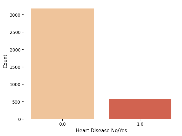
# Checking balance of outcome variable
target_count = df_scaled.TenYearCHD.value_counts()
print('Class 0:', target_count[0])
print('Class 1:', target_count[1])
print('Proportion:', round(target_count[0] / target_count[1], 2), ': 1')
Output:
Class 0: 3178
Class 1: 571
Proportion: 5.57 : 1
Figure 1. Frequency counts of heart disease outcome

"""
Valancing Instances
We can use the undersampling technique to reduce the instances of the overrepresented class in the dataset.
In our scenario, these methods will bring down the number of fraudulent transactions in our data to a
balanced ratio of approximately 50:50. By ensuring equal representation, we prevent classification
algorithms from being biased towards the majority class. This prevents misleading results where it may
appear that your algorithm is performing exceptionally well (overfitting), while it is actually just
consistently predicting the majority class.
We can achieve a balance between the majority and minority classes by randomly selecting observations
from the majority class and removing them. Another method is matching where X features of the minor
class are matched with those of the major class. Matching is computationally difficult but useful
when the length (instances) of the minor class is very small (< 100).
"""
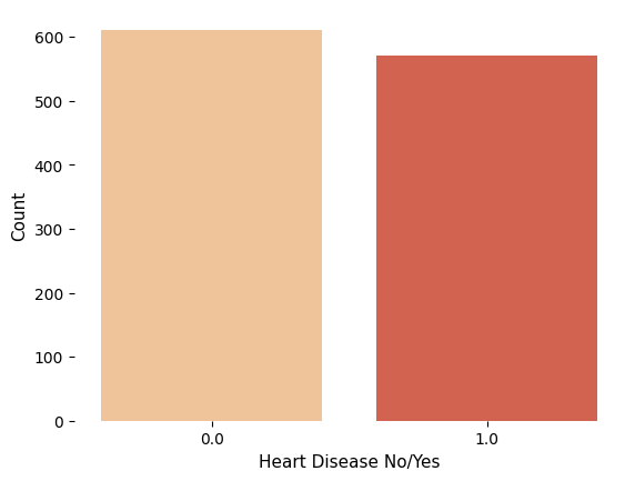
# First seperate the dataset by class and randomly select 611 case from the major class.
shuffled_df = df_scaled.sample(frac=1, random_state=4)
CHD_df = shuffled_df.loc[shuffled_df['TenYearCHD'] == 1]
non_CHD_df = shuffled_df.loc[shuffled_df['TenYearCHD'] == 0].sample(n=611, random_state=42)
# Then combine the two datasets.
# Concatenate both dataframes again
normalized_df = pd.concat([CHD_df, non_CHD_df])
#Define y & X again
y = normalized_df['TenYearCHD']
X = normalized_df.drop(['TenYearCHD'], axis = 1)
Split to Train and Test subsets.
# divide train test: 80 % - 20 %
X_train, X_test, y_train, y_test = train_test_split(X, y, test_size = 0.2, random_state=29)
# plot new count
sns.countplot(normalized_df, x='TenYearCHD', palette="OrRd")
plt.box(False)
plt.xlabel('Heart Disease No/Yes', fontsize=11)
plt.ylabel('Count',fontsize=11)
plt.show()
Figure 2 Balanced CHD outcomes

Model Pipeline
A model pipeline refers to a sequential and systematic process in which machine learning models are developed, trained, evaluated, and deployed. It is an essential framework that ensures the efficient transformation of raw data into valuable insights or predictions. The model pipeline begins by defining clear objectives and identifying relevant variables for analysis. Data preprocessing techniques such as cleaning, normalization, and feature extraction are then applied to enhance the quality of input data.
Once prepared, this dataset is split into training and testing sets to develop a suitable model architecture using various algorithms like decision trees or neural networks. During the training phase, the chosen algorithm learns patterns from labeled data through iterative optimization processes until it achieves desirable performance metrics such as accuracy or loss minimization. Afterward, the model's performance is evaluated on unseen test data to assess its generalizability and potential biases present in its predictions. If deemed satisfactory, the model proceeds towards deployment where it can make real-time predictions on new incoming data with minimal human intervention.
Throughout this entire process of building a robust model pipeline, diligent documentation helps maintain transparency regarding methodologies used and facilitate collaboration among multiple stakeholders involved in creating effective predictive solutions for complex problems across diverse industries such as healthcare diagnostics or financial forecasting.
# Import libraries
from sklearn.pipeline import Pipeline
from sklearn.linear_model import LogisticRegression
from sklearn.svm import SVC
from sklearn.tree import DecisionTreeClassifier
from sklearn.neighbors import KNeighborsClassifier
from sklearn.model_selection import GridSearchCV
from sklearn.model_selection import cross_val_score
# Testing the accuracy of each model using Pipeline
classifiers = [LogisticRegression(), SVC(), DecisionTreeClassifier(), KNeighborsClassifier(2)]
for classifier in classifiers:
    pipe = Pipeline(steps=[('classifier', classifier)])
    pipe.fit(X_train, y_train)
    print("The accuracy score of {0} is: {1:.2f}%".format(classifier,
        (pipe.score(X_test, y_test)*100)))
Accuracy:
Accuracy indicates how often the classifier is correct? Accuracy = (True Positive + True Negative)/total
The accuracy score of LogisticRegression() is: 68.35%
The accuracy score of SVC() is: 65.82%
The accuracy score of DecisionTreeClassifier() is: 54.01%
The accuracy score of KNeighborsClassifier(n_neighbors=2) is: 56.12%
Continue to Chapter 5. Model Evaluation